Why Your Model is Failing (Hint: It’s Not the Architecture)

A bug-proof guide to lazy loading, smart transforms, and handling messy production data in PyTorch.

We’ve all been there. You spend days tuning hyperparameters and tweaking your architecture, but the loss curve just won’t cooperate. In my experience, the difference between a successful project and a failure is rarely the model architecture. It’s almost always the data pipeline.

I recently built a robust data pipeline solution for a private work project. While I can’t share that proprietary data due to privacy reasons, the challenges I faced are universal: messy file structures, proprietary label formats, and corrupted images.

To show you exactly how I solved them, I’ve recreated the solution using the Oxford 102 Flowers dataset. It is the perfect playground for this because it mimics real-world messiness: over 8,000 generically named images with labels hidden inside a proprietary MATLAB (.mat) file rather than nice, clean category folders.

Here is the step-by-step guide to building a bugproof PyTorch data pipeline that handles the mess so your model doesn’t have to.

1. The Strategy: Lazy Loading & The Off-by-One Trap

If you can’t reliably load your data, nothing else matters.

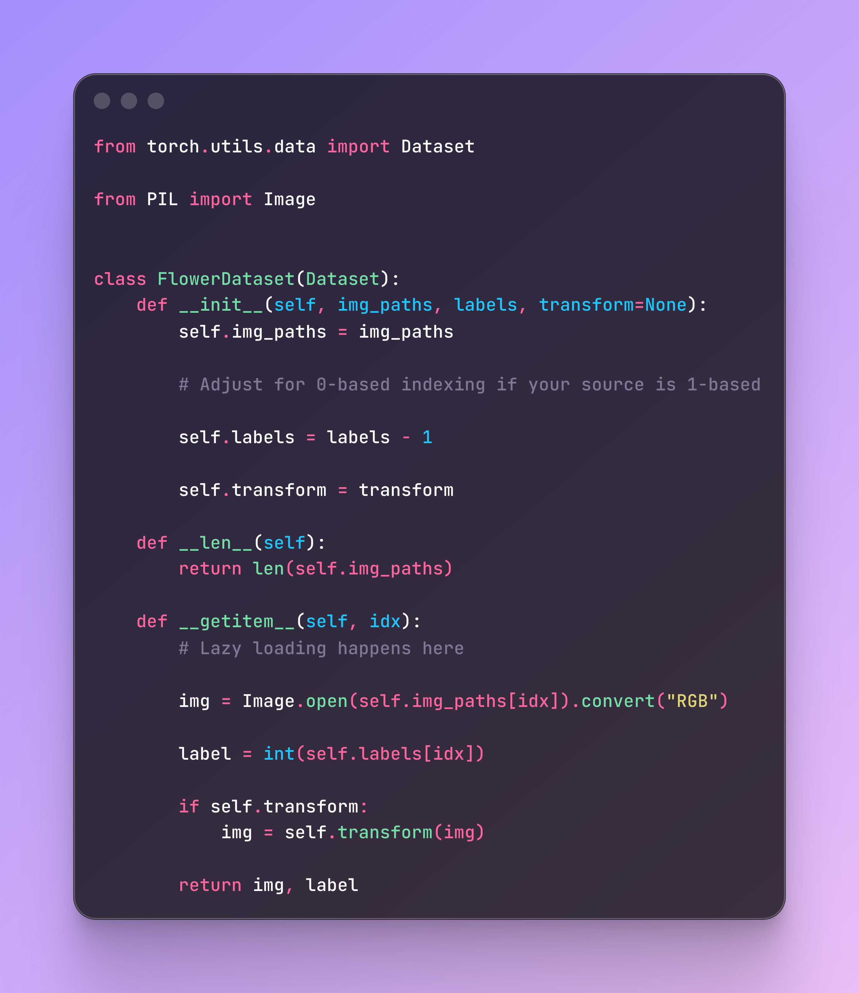
For this pipeline, I built a custom PyTorch Dataset class focused on lazy loading. Instead of loading all 8,000+ images into RAM at once, we store only the file paths during setup (__init__) and load the actual image data on-demand (__getitem__).

A critical lesson learned: Watch out for indexing errors. The Oxford dataset uses 1-based indexing for its labels, but PyTorch expects 0-based indexing. Catching this off-by-one error early saves you from training a perpetually confused model.

The Dataset Skeleton

Here is the core structure we need to implement:

2. Consistency: The Pre-processing Pipeline

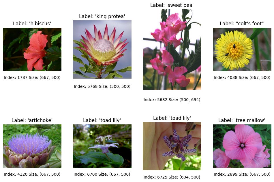
Real-world data is rarely consistent. In the Flowers dataset, images have wildly different dimensions (e.g., 670x500 vs 500x694). PyTorch batches require identical dimensions, so we need a rigorous transform pipeline.

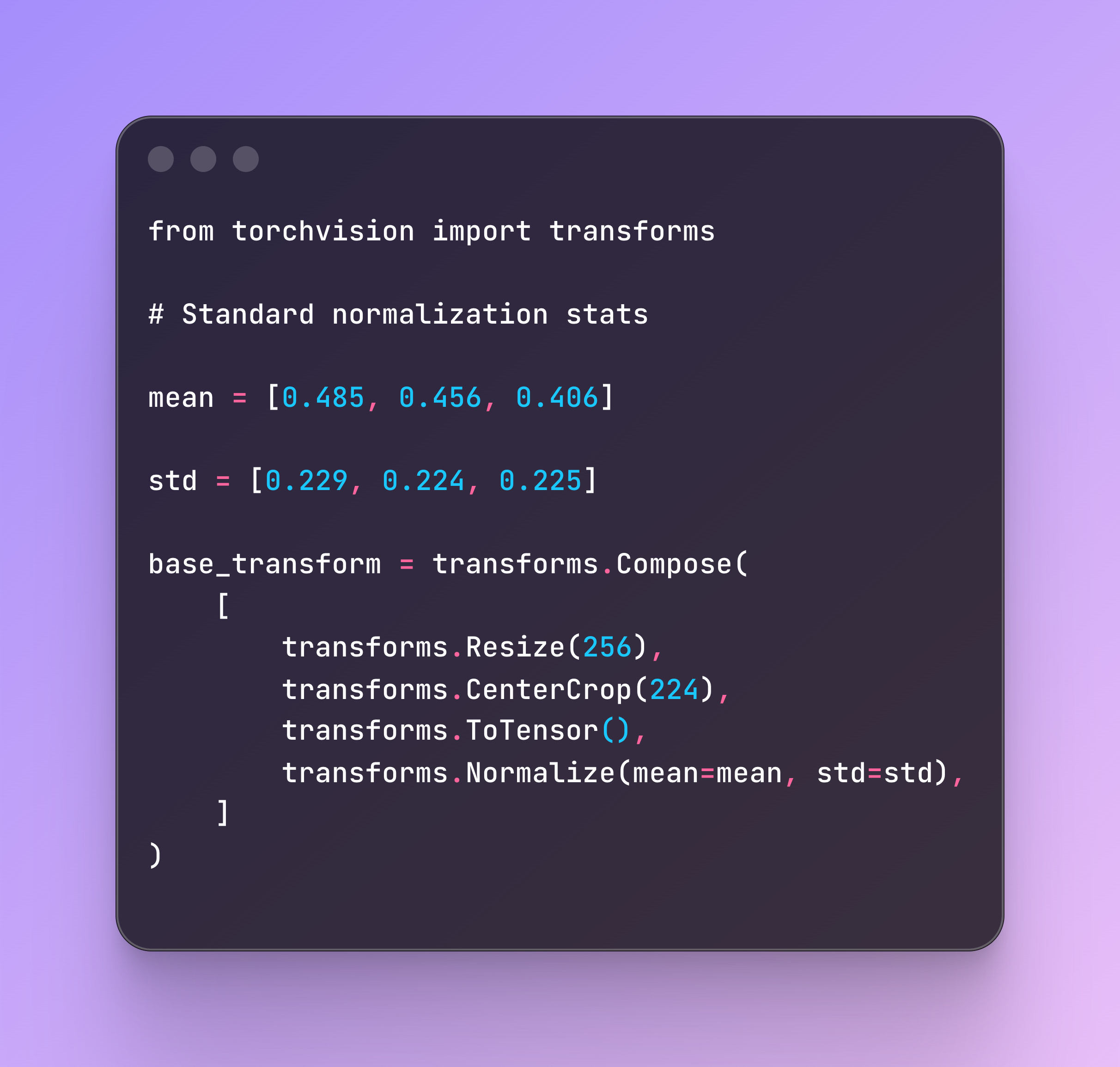
I strictly avoid simple resizing, which distorts the image. Instead, I use a Resize on the shorter edge to preserve the aspect ratio, followed by a CenterCrop to get our uniform square. Finally, we convert to tensors and normalize pixel intensity from 0-255 down to 0-1.

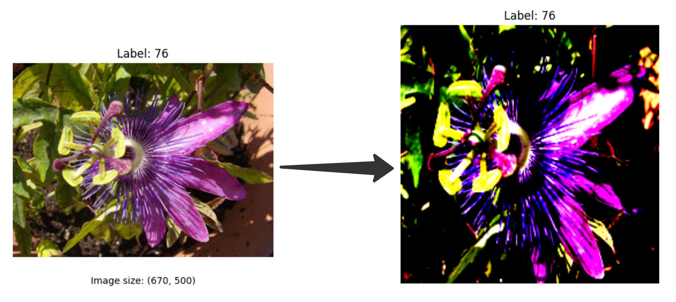
And here is the output for a sample image:

3. Augmentation: Endless Variation, Zero Extra Storage

One of the biggest advantages of PyTorch’s on-the-fly augmentation is that it provides endless variation without taking up extra storage.

By applying random transformations (flips, rotations, and color jitters) only when the image is loaded during training, the model sees a slightly different version of the image every epoch. This forces the model to learn essential features like shape and color rather than memorizing pixels.

Note: Always disable augmentation for validation and testing to ensure your metrics reflect actual performance improvements.

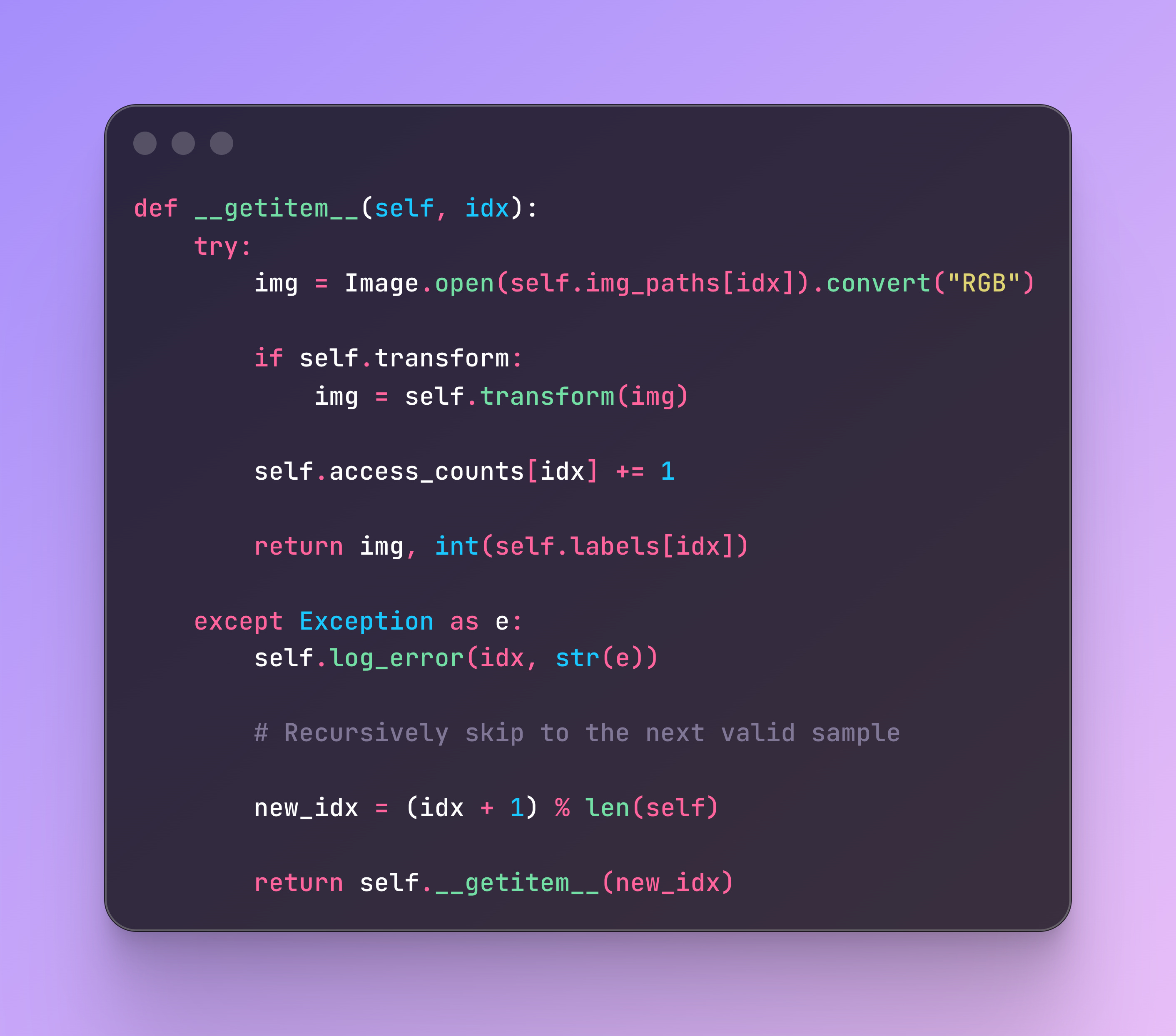
4. The Bugproof Pipeline: Handling Corrupted Data

This is the part that usually gets overlooked in tutorials but is vital in production. A single corrupted image can crash a training run hours after it starts.

To fix this, we update the __getitem__ method to be resilient. If it encounters a bad file (corrupted bytes, empty file, etc.), it shouldn’t crash. Instead, it should log the error and recursively call itself to fetch the next valid image.

Here is the pattern I use:

5. Telemetry: Know Your Data

Finally, I added basic telemetry to the pipeline. By tracking load times and access counts, you can identify if specific images are dragging down your training throughput (e.g., massive high-res files) or if your random sampler is neglecting certain files.

In my implementation, if an image takes longer than 1 second to load, the system warns me. After training, I print a summary like:

• Total images: 8,189

• Errors encountered: 2

• Average load time: 7.8 ms

Summary

If you are shipping models to production, you need to invest as much time in your data pipeline as you do in your model architecture.

By implementing lazy loading, consistent transforms, on-the-fly augmentation, and robust error handling, you ensure that your sophisticated neural network isn’t being sabotaged by a broken data strategy.